WaveSpectra2DSplitFit’s documentation!
Python Package for Ocean Wave Spectra 2D Splitting, Fitting and Reconstruction
Introduction
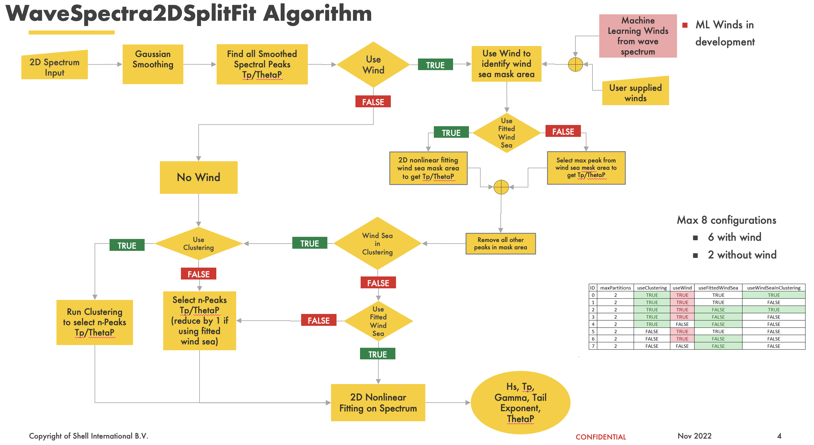
The main purpose of this package is to find parameters of JONSWAP wave spectra with spreading that, when recombined, best match the input 2D frequency direction wave spectra. Given a 2D wave spectrum S(f,theta), the package finds parameters of multiple JONSWAP partitions including wave spreading (i.e. Hs, Tp, Gamma, Tail exponent, ThetaP).
The aim of the package is to provide an industry wide approach to derive usable wave spectral parameters that provide the best possible reconstruction of the input wave spectrum. The method is designed to be tunable, but robust in the default configuration. A large number of observed and numerically modelled datasets have been tested during the creation and validation of the method.
It is the intention that the package will be used by consultants and weather forecastors to improve the descriptions of the ocean wave partitions for use in operations and engineering applications. It provides the metocean engineer with a robust way to separate swells and wind seas in the development of metocean design fatigue, operational and extreme criteria.
Usage
Provide a 2D wave spectrum defined with frequencies [Hz], directions [degrees] and spectral densities [m^2 / (Hz.rad)] and define the maximum number of wave partitions.
Run the fitting
Each fitted spectrum is defined by: Hs, Tp, JONSWAP Gamma, JONSWAP SigmaA, JONSWAP SigmaB, JONSWAP Tail Exponent, ThetaP
Fitting returns sets of spectrum parameters for up to maximum number of parameters
NB. JONSWAP SigmaA and SigmaB are fixed at 0.07 and 0.09
import numpy as np
from wavespectra2dsplitfit.S2DFit import readWaveSpectrum_mat
filename = 'data/ExampleWaveSpectraObservations.mat'
f, th, S, sDate = readWaveSpectrum_mat(filename)
S = S * np.pi/180 # convert from m^2/(Hz.rad) to m^2/(Hz.deg)
# Setup fitting configuration - simple example with no wind (also usually best setup with no wind)
tConfig = {
'maxPartitions': 3,
'useClustering': True,
'useWind': False,
'useFittedWindSea': False,
'useWindSeaInClustering': False,
}
# Just do the first spectrum
from wavespectra2dsplitfit.S2DFit import fit2DSpectrum
specParms, fitStatus, diagOut = fit2DSpectrum(f[0], th[0], S[0,:,:], **tConfig)
print(specParms, fitStatus)
for tSpec in specParms:
print("===== PARTITION =====")
print("Hs = ",tSpec[0])
print("Tp = ",tSpec[1])
print("Gamma = ",tSpec[2])
print("Sigma A = ",tSpec[3])
print("Sigma B = ",tSpec[4])
print("Tail Exp = ",tSpec[5])
print("ThetaP = ",tSpec[6])
print("===== FITTING OUTCOME =====")
print(f"Fitting successful: ",fitStatus[0])
print(f"RMS error of fit: ",fitStatus[1])
print(f"Number of function evalutions: ",fitStatus[2])
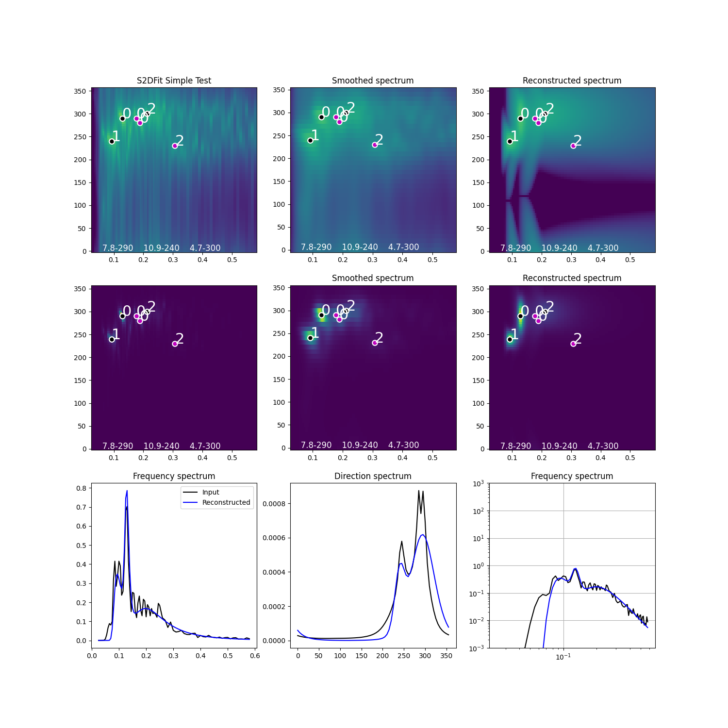
from wavespectra2dsplitfit.S2DFit import plot2DFittingDiagnostics
f, th, S, f_sm, th_sm, S_sm, wsMask, Tp_pk, ThetaP_pk, Tp_sel, ThetaP_sel, whichClus = diagOut
plot2DFittingDiagnostics(
specParms,
f, th, S,
f_sm, th_sm, S_sm,
wsMask,
Tp_pk, ThetaP_pk, Tp_sel, ThetaP_sel, whichClus,
tConfig['useWind'], tConfig['useClustering'],
saveFigFilename = 'test',
tag = "S2DFit Simple Test"
)
Example Result:
$ python test.py
 Optimization terminated successfully.
          Current function value: 0.082135
          Iterations: 1082
          Function evaluations: 1733
 [[0.5859285326910995, 4.716981132075468, 1.0000053476007895, 0.07, 0.09, -4.234276488479486, 300.0, 4.716981132075468], [0.6129423521749234, 7.812499999999995, 5.970526837658344, 0.07, 0.09, -5.140143260428807, 290.0, 7.812499999999995], [0.4047506936099149, 10.869565217391298, 1.0000041524068202, 0.07, 0.09, -15.401874257914326, 240.0, 10.869565217391298]] [True, 0.08213522716322981, 1733]
 ===== PARTITION =====
 Hs =  0.5859285326910995
 Tp =  4.716981132075468
 Gamma =  1.0000053476007895
 Sigma A =  0.07
 Sigma B =  0.09
 Tail Exp =  -4.234276488479486
 ThetaP =  300.0
 ===== PARTITION =====
 Hs =  0.6129423521749234
 Tp =  7.812499999999995
 Gamma =  5.970526837658344
 Sigma A =  0.07
 Sigma B =  0.09
 Tail Exp =  -5.140143260428807
 ThetaP =  290.0
 ===== PARTITION =====
 Hs =  0.4047506936099149
 Tp =  10.869565217391298
 Gamma =  1.0000041524068202
 Sigma A =  0.07
 Sigma B =  0.09
 Tail Exp =  -15.401874257914326
 ThetaP =  240.0
 ===== FITTING OUTCOME =====
 Fitting successful:  True
 RMS error of fit:  0.08213522716322981
 Number of function evalutions:  1733
An example of the input and output reconstructed spectrum are shown in the image below.